Rune’s recent talk on layered procedural generation has got me thinking about procedural generation again, so I wanted to share a technique I found about doing a uniform distribution of points on an infinite plane. I assumed this would be a well known thing, but I couldn’t find any references elsewhere.

Skip to Results to see the final thing.

What is a Uniform Distribution?

A uniform distribution is a probability distribution where the location of a single point is picked and every location in a given area is equally likely.

It’s the most common distributions used – most programming languages give a pseudo-random number generator built in that gives a uniform distribution of numbers between 0 and 1, often simply called random() or something.

Given a uniform generator with range 0 to 1, you can make a lot of other uniform generators:

• To uniformly pick a point in the range a to b, simply compute random() * (b - a) + a
• To uniformly pick a point in a rectangle, generate two random points in ranges, one for the x-axis and one for the y-axis.
• To uniformly pick a point in a cube, use the same trick as rectangle, but for three axes.
• To uniformly pick a point in an irregular shape, you can generate points in a bounding box, repeating until you find the first one actually inside the shape,

More commonly, in PCG, you uniformly distribute \(N\) points, which simply means uniformly picking each of them independently.

Uniform distributions are popular because of their simplicity, and they have a distinctive look: you can see there are often randomly very dense or empty patches.

Infinite PCG?

Nothing in computing is literally infinite. The computer itself can only hold a finite amount of stuff in memory. What infinite really means is endless – we’ll never run out of stuff to show the user, as they scroll around an “infinite” map. So we want something that can generate pieces of a larger map on-demand, with each of the pieces being consistent with each other.

The general approach for any infinite map generator is chunking. We cut the entire infinite plane up into equal sized squares, called chunks, and evaluate the each separately. Each chunk has a seed derived from its position, so we don’t need to store calculated chunks – we can just regenerate the exact same result for that chunk if we ever need to return to the same location.

Sometimes there are complexities about how chunks interact with each other, but in this article this won’t come up.

Jittered Grids

Ok, so it seems like the solution is obvious. Split the map up into chunks, then uniformly generate a point in each chunk.

This solution is simple, and looks good. It’s a popular technique called jittered grids. But it’s not actually truly uniform. Because we have exactly one point per chunk, it’s impossible to ever get an area which is completely empty of chunks, or where they have clustered together really densely, which I consider the defining aspect of a uniform distribution.

You can improve on this by using larger chunks, and generating proportionally more points per chunk.

But you’ll never get the exact distribution I want, and larger chunks are less efficient to evaluate anyway.

So what is the exact distribution?

A formal definition

Note: This section is a little maths heavy. Just read the first bit and move on if it’s not interesting.

The intuition is that an infinite uniform distribution of points should resemble as closely as possible the uniform distribution for a really large rectangle.

Because we are thinking about infinite areas and rectangles of varying sizes, instead of talking about generating \(N\) points, let’s talk about distributing points with a fixed density, \(\rho\) (the greek letter “rho”). I.e. for a given rectangle, we pick the number of points equal to \(\rho * area(rectangle) \), rounding to the nearest integer.

To formalise the idea of a really large rectangle, we’re actually going to imagine a series of rectangles, each larger than the last. By analysing what properties this series has, particularly as we get to larger and larger rectangles, allows us to extrapolate to the infinite case. This is called a “limiting process”, and I discuss it in a bit more detail in this article.

E.g. for \(\rho = 1\). Start with a 1×1 rectangle, which we distribute 1 point in. Then a 2×2 rectangle that we distribute 4 points in. Then a 3×3 rectangle that we distribute 9 points in. And so on.

We can now do an analysis of the properties of the distribution, as the rectangles grow larger and larger. For each rectangle, let’s cut out a 1×1 sub-rectangle, so we have something to directly compare.

So for the \(N\)th rectangle, it has area \(N^2\), and will have \(\rho N^2\) points in it. Each point has an independent \(1 / N^2\) chance of landing in the 1×1 sub-rectangle. That means that the count of points that are in that sub-rectangle has a binomial distribution, \( B(\rho N^2, 1/N^2) \).

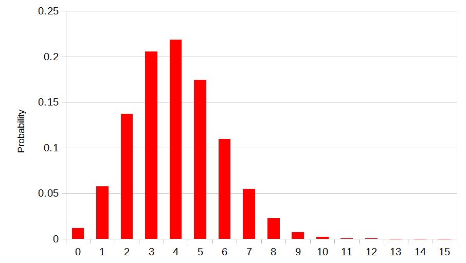
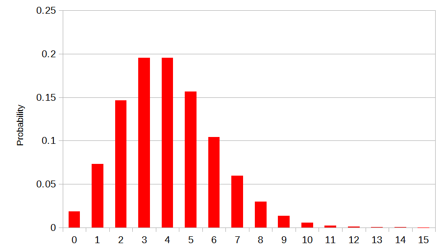
The binomial distribution looks like a long tailed hump – while it’s possible to get 0 points, or \(\rho N^2\) points, right at the edges of the hump, it’s much more likely to get a number around \(\rho N^2 \times 1/N^2 = \rho \).

As \(N\) increases, the shape of the hump stabilises, and it starts to change less and less. It is a known result that Binomial distributions like this converge to a specific distribution, known as the Poisson distribution¹.

So this is what we’ll use for the true infinite case, the largest of all large rectangles. We’ll specifically conclude: For an infinite uniform distribution with density \(\rho\), the count of points found inside any shape of area \(A\) is distributed as \(Poisson(\rho A)\).

Formally, this sort of distribution is known as a Poisson Point Process.

My Implementation

Armed with this fact, the algorithm is very simple. We use on chunking, and lazy evaluation, and evaluate each chunk independently².

There’s two steps for generating the points in a chunk:

• Randomly pick the number of points in the chunk (with Poisson distribution)
• Randomly distribute that number of points in the chunk (with uniform distribution)

The size and shape of the chunks doesn’t matter, but it’s convenient for computations to pick square chunks of size \(1/\sqrt{\rho} \). Then the Poisson distribution always uses parameter 1 (i.e. the average number of points in the chunk is 1, like a jittered grid).

Here’s the same thing in pseudo code:

DENSITY=1.3
CHUNK_SIZE=10

def points_in_chunk(x, y):
    # Use deterministic random numbers
    seed = hash([x, y])
    r = PRNG(seed)
    # Randomly sample the poisson distribution
    L = CHUNK_SIZE * CHUNK_SIZE * DENSITY
    n = sample_poisson(r, L)
    # Generate n random points in the area of this chunk
    minx = x * CHUNK_SIZE
    maxx = minx + CHUNK_SIZE
    miny = y * CHUNK_SIZE
    maxy = miny + CHUNK_SIZE
    return [
        (sample_uniform(r, minx, max), sample_uniform(r, miny, maxy)
        for i in range(n)
    ]

def sample_uniform(r, min, max):
    return r.next_double() * (max - min) + min

STEP = 500 # suitable for double precision floats
def sample_poisson(r, L):
    # Ported from wikipedia, see https://en.wikipedia.org/wiki/Poisson_distribution
    left = L
    k = 0
    p = 1
    while True:
        k += 1
        p *= r.next_double()
        while p < 1 and left > 0:
            if left > STEP:
                p *= exp(STEP)
                left -= STEP
            else:
                p *= exp(left)
                left = 0
        if p <= 1: break
    return k - 1 

Results